
Waveforms in KMAX
Posted by Karl Auerbach /
Real network conditions are rarely static. Real life networks suffer transient conditions – congestion builds up and dissipates, tree branches wave in the wind across radio links, long distance routing paths change, VoIP call trunks are filled with more calls during working hours than during the evening. Even something as small as a person standing near a wi-fi access point can change the carrying capacity of a network.
KMAX and our Maxwell Pro can emulate these kinds of changes.
Many network emulators, including KMAX, can perform high-frequency variations. This is typically called “jitter” and involves a random process (a “stochastic” process) to rapidly vary some impairment parameter (such as packet delay) over some short period of time (typically milliseconds) and according to a statistically defined probability function (such as a uniform or Gaussian distribution.)
But the kinds of changes described above are low frequency variations. Network congestion, for instance, builds and fades over periods of seconds or longer. Environmental noise (such as wind blowing branches in front of a satellite ground station dish) occur and re-occur over spans of seconds. And longer cycles (such as congestion of VoIP lines) tend to follow the hours of the business day.
Most network emulators do not have ways to create these kinds of low-frequency changes. But KMAX can.
Many of the impairment parameters in KMAX can be modulated using a “Waveform”.
A KMAX waveform adjusts a given parameter over periods that can range from a second to many hours (or longer).
A waveform is composed of repeating cycles. Each cycle drives its impairment parameter from a starting value, through a sequence of changes over time, and then back to the starting value. The cycles repeat for as long as waveform processing is enabled.
Waveforms can be an extremely powerful tools. For example, consider a user who is trying to test some TCP code to see how well it handles congestion conditions. It would be very useful to set up a sequence of waves that begin by allowing TCP packets to cross the net with minimal delay for a minute or two, then slowly increase the delay (and perhaps the packet loss) gradually over a period of couple of minutes, and then suddenly drop the delay (and packet loss) back to the original minimal delay. (This is not a hypothetical test – over the years several TCP implementations have faced this kind of test and have come up wanting.)
Let’s look at a typical KMAX waveform – we will use the one for delay:

The first thing to notice is that the screen is divided into three major parts:
At the top are controls to enable the waveform and to put it into motion.
In the middle are four gray areas, each defining a different method of varying the parameter:
Manual – This is essentially a no-operation setting. It means that the waveform does not change the impairment setting that comes from the main screen for that particular parameter.
Pulse Model – This is the easiest and most common way to define a waveform cycle.
Python expression – This lets you define use a Python language expression to define the Y value (that’s the up/down axis) of the graph.
List of value:duration pairs – Here you can draw the graph as a series of X:Y point coordinates.
At the bottom are a pair of graphs showing how a proposed waveform looks and how it is running in practice.
Let’s dig into the Pulse Model.
A single pulse cycle is defined by six parameters:
Baseline Value
Target Value
Lead Time
Onset Time
Hang Time
Fall Time
The units for the Baseline and Target parameters will be different for various types of impairments. The various Time parameters will be in seconds or milliseconds.
Imagine a roller-coaster ride at an amusement park. You get in at the starting level – that’s the Baseline. Then the ride starts and runs on the level track for a while. That’s the Lead time. Then you go up. The time it takes to go up that rise to the top is the Onset time, and the height at the top is the Target. You may stay at the top for a while – that’s the Hang time. Then there is the drop back to the baseline. The duration of that drop is the Fall time.
The shorter the Onset and Fall times the steeper the angle of ascent from the Baseline to the top (Target) value or the steeper the angle of the descent.
You can see how the waveform will look by clicking on the Preview control. In the screen shot below you can see how the six pulse model parameters create the shape shown in the Preview Graph.
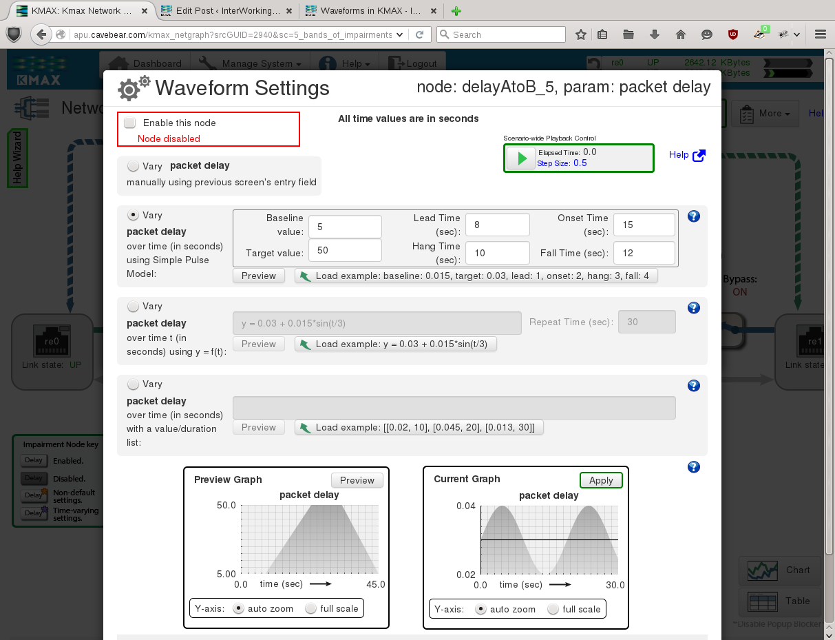
Use the Apply control to enable the waveform.
Waveforms do not run until you activate them by clicking on the green triangle near the top of the screen.
You may have multiple wave forms in operation at the same time. They run together – in other words they are all stopped and started together (you can’t run just one all by itself – but you can effectively turn off the ones you don’t want by using the “Manual” setting on the ones you don’t want to use.)